From Marketing Mix Models to Custom Bayesian GAMs: Extending PyMC-Marketing’s Core#

Introduction#

While PyMC-Marketing is widely recognized for its advanced Marketing Mix Modeling (MMM) capabilities, its true potential extends far beyond traditional MMM frameworks. At its core, PyMC-Marketing provides a flexible and composable architecture that enables the construction of complex probabilistic models—particularly generalized additive models (GAMs)—within the Bayesian paradigm. By leveraging PyMC’s expressive modeling syntax and the modular structure of PyMC-Marketing, everyone can integrate nonlinear transformations, hierarchical priors, auto-regressive dynamics with just a few lines of code or to define their own custom transformations that reflect domain-specific knowledge and data-driven insights. In doing so, PyMC-Marketing becomes not only a framework for marketing optimization but also a general-purpose engine for building interpretable Bayesian GAMs. This flexibility makes it an invaluable tool for anyone seeking to combine causal reasoning, functional flexibility, and probabilistic inference in a coherent modeling workflow.

This allows researchers and analysts to move seamlessly from standard MMMs to fully specified graphical models that capture richer causal and functional relationships across variables.

In the following notebook, we’ll showing you several of these functionalities. You can read more about individual components and how to build MMM’s in the components notebook.

Import libraries#

from __future__ import annotations

import time
import warnings
from collections.abc import Sequence
from copy import deepcopy

import arviz as az
import matplotlib.pyplot as plt
import numpy as np
import pandas as pd
import pymc as pm
import xarray as xr
from pymc_extras.prior import Prior, create_dim_handler

from pymc_marketing.mmm import (
    GeometricAdstock,
    LogisticSaturation,
    NoAdstock,
    NoSaturation,
)
from pymc_marketing.mmm.components.base import Transformation
from pymc_marketing.mmm.multidimensional import MMM
from pymc_marketing.special_priors import LogNormalPrior, MaskedPrior

OMP: Info #276: omp_set_nested routine deprecated, please use omp_set_max_active_levels instead.
/Users/carlostrujillo/Documents/GitHub/pymc-marketing/pymc_marketing/mmm/multidimensional.py:216: FutureWarning: This functionality is experimental and subject to change. If you encounter any issues or have suggestions, please raise them at: https://github.com/pymc-labs/pymc-marketing/issues/new
  warnings.warn(warning_msg, FutureWarning, stacklevel=1)

Setting notebook#

warnings.filterwarnings("ignore", category=UserWarning)

seed: int = sum(map(ord, "pymc-marketing is more than just a marketing model"))

az.style.use("arviz-darkgrid")
plt.rcParams["figure.figsize"] = [12, 7]
plt.rcParams["figure.dpi"] = 100
plt.rcParams["xtick.labelsize"] = 10
plt.rcParams["ytick.labelsize"] = 8

%load_ext autoreload
%autoreload 2
%config InlineBackend.figure_format = "retina"

Data generation process#

For the following examples, we won’t build a large structural process, since the goal of this notebook is simply to showcase the library’s capabilities. Instead, we’ll generate a few time series following random walks and define a simple linear target variable that depends on the number of created drivers.

The series can be viewed as marketing variables or drivers aimed at a specific target. As we move through the notebook, we’ll generate numerous examples of potential datasets that can be used with each of the models.

def random_walk(mu, sigma, steps, lower=None, upper=None, seed=None):
    """
    Generate a bounded random walk with specified mean and standard deviation.

    Parameters
    ----------
    mu : float
        Target mean of the random walk
    sigma : float
        Target standard deviation of the random walk
    steps : int
        Number of steps in the random walk
    lower : float, optional
        Lower bound for the random walk values
    upper : float, optional
        Upper bound for the random walk values
    seed : int, optional
        Random seed for reproducibility

    Returns
    -------
    np.ndarray
        Random walk array with specified mean, std, and bounds
    """
    # if seed none then set 123
    if seed is None:
        seed = 123
    # Create a random number generator with the given seed
    rng = np.random.RandomState(seed)

    # Start from the target mean
    walk = np.zeros(steps)
    walk[0] = mu

    # Generate the walk step by step with bounds checking
    for i in range(1, steps):
        # Generate a random increment using the seeded RNG
        increment = rng.normal(0, sigma * 0.1)  # Scale increment size

        # Propose next value
        next_val = walk[i - 1] + increment

        # Apply bounds if specified
        if lower is not None and next_val < lower:
            # Reflect off lower bound
            next_val = lower + (lower - next_val)
        if upper is not None and next_val > upper:
            # Reflect off upper bound
            next_val = upper - (next_val - upper)

        # Final bounds check (hard clipping as backup)
        if lower is not None:
            next_val = max(next_val, lower)
        if upper is not None:
            next_val = min(next_val, upper)

        walk[i] = next_val

    # Adjust to match target mean and std while respecting bounds
    current_mean = np.mean(walk)
    current_std = np.std(walk)

    if current_std > 0:
        # Center around zero, scale to target std, then shift to target mean
        walk_centered = (walk - current_mean) / current_std * sigma + mu

        # Apply bounds again after scaling
        if lower is not None:
            walk_centered = np.maximum(walk_centered, lower)
        if upper is not None:
            walk_centered = np.minimum(walk_centered, upper)

        walk = walk_centered

    return walk

n_days = 365
n_years = 6
n_observations = n_days * n_years
min_date = pd.to_datetime("2022-01-01")
max_date = min_date + pd.Timedelta(days=n_observations) - pd.Timedelta(days=1)
date_range = pd.date_range(start=min_date, end=max_date, freq="D")
df = pd.DataFrame(data={"date_week": date_range})

x1 = random_walk(
    mu=500, sigma=50, steps=n_observations, lower=10, upper=1000, seed=seed + 1
)
x2 = random_walk(
    mu=300, sigma=100, steps=n_observations, lower=10, upper=1000, seed=seed + 2
)
x3 = random_walk(
    mu=600, sigma=80, steps=n_observations, lower=10, upper=1000, seed=seed - 3
)
x4 = random_walk(
    mu=1000, sigma=100, steps=n_observations, lower=10, upper=3000, seed=seed - 1
)

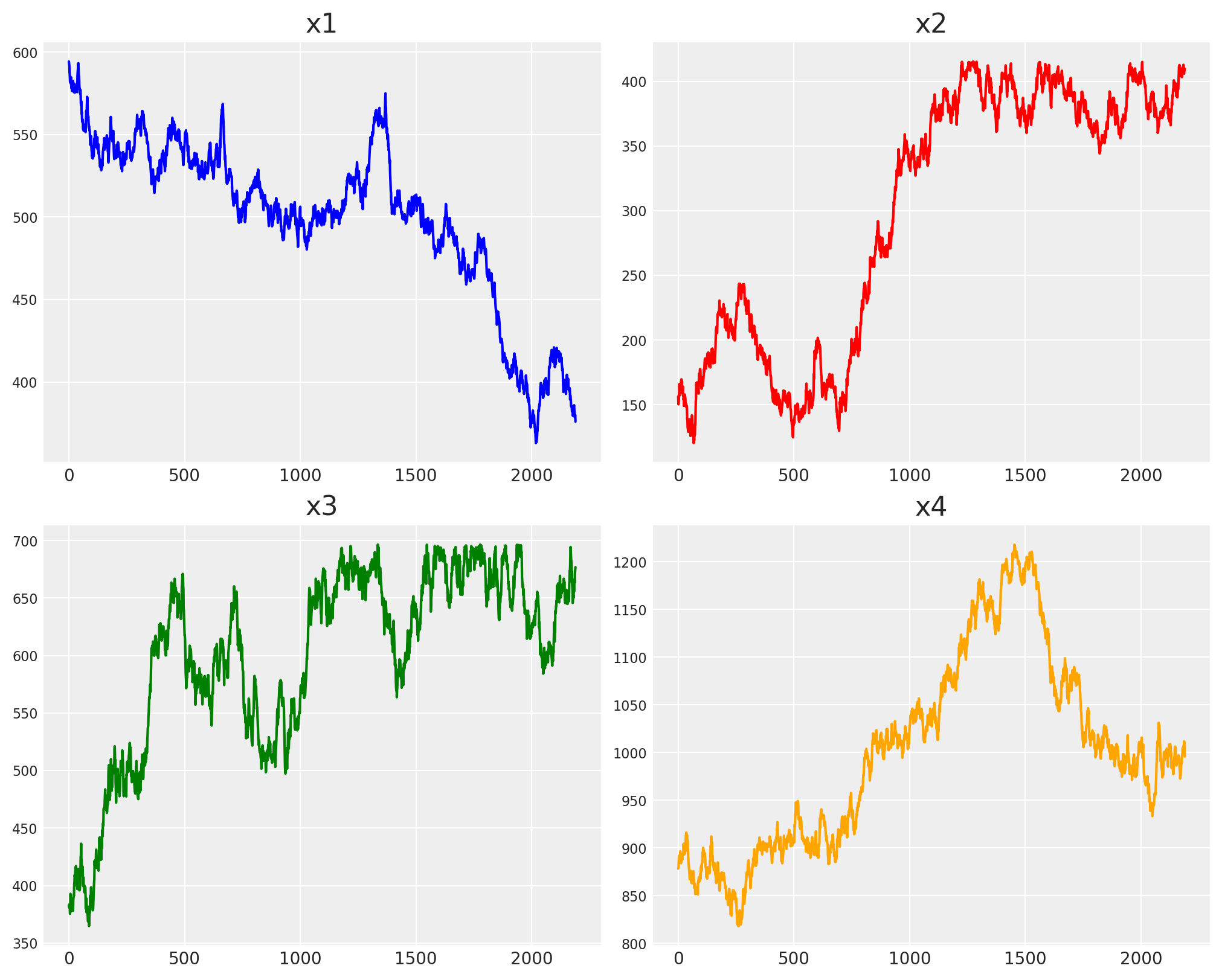
Great, let’s visualize our time series!

fig, axs = plt.subplots(2, 2, figsize=(10, 8))
axs[0, 0].plot(x1, color="blue")
axs[0, 0].set_title("x1")
axs[0, 1].plot(x2, color="red")
axs[0, 1].set_title("x2")
axs[1, 0].plot(x3, color="green")
axs[1, 0].set_title("x3")
axs[1, 1].plot(x4, color="orange")
axs[1, 1].set_title("x4")
plt.show()

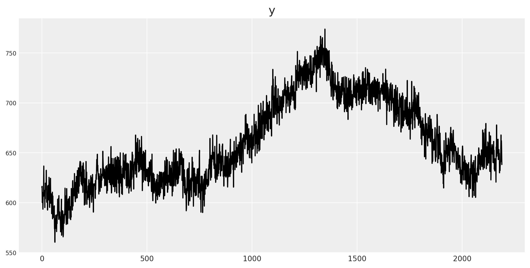
../../_images/78d16aab4fbf49459517a31c6a656398da70c59cb7670a4ef8f650a83f888015.png

We’ll build a simple linear model based on these four factors. You can think of them as representing impressions, spend, or any other typical marketing variable, while the target could correspond to outcomes such as revenue, installs, site registrations, or purchases.

intercept = 100
noise = np.random.normal(0, 10, n_observations)
y = x1 * 0.5 + x2 * 0.3 + x3 * 0.2 + x4 * 0.1 + intercept + noise

df["x1"] = x1
df["x2"] = x2
df["x3"] = x3
df["x4"] = x4
df["y"] = y

fig, ax = plt.subplots(figsize=(10, 5))
ax.plot(y, color="black")
ax.set_title("y")
plt.show()

../../_images/2fd30072fb5fe83e83aa7b00c27611a0c56d70271809458fb9e50a38a6f61332.png

We put all the data together in the same dataset.

df.head()

	date_week	x1	x2	x3	x4	y
0	2022-01-01	594.252746	156.373242	382.601781	878.408481	615.369383
1	2022-01-02	592.904201	150.323907	381.212926	878.912259	616.370832
2	2022-01-03	591.613607	151.588310	383.524140	881.134924	600.228101
3	2022-01-04	587.537071	154.705806	381.000766	889.327060	601.415660
4	2022-01-05	585.676798	158.286095	379.739704	886.491672	601.148165

Sampler settings#

We’ll make a set of predifine sampler settings for all our models.

sample_kwargs = {
    "tune": 800,
    "draws": 200,
    "chains": 2,
    "random_seed": seed,
    "target_accept": 0.84,
}

Simple Linear Model#

To begin, we’ll construct a basic linear model using the MMM class. This example demonstrates how PyMC-Marketing can easily represent a standard linear regression.

In this setup, the target variable \(Y_t\) is modeled as a linear combination of several predictors \(X_{i,t}\), each weighted by its corresponding coefficient \(b_i\), plus a random error term \(\varepsilon_t\):

\[ Y_t = \sum_{i=1}^{I} b_i X_{i,t} + \varepsilon_t \]

Here:

\(Y_t\) represents the target at time \(t\) (e.g., revenue, installs, or registrations),
\(X_{i,t}\) are the explanatory variables (e.g., impressions, spend, or other marketing drivers),
\(b_i\) are the channel-specific coefficients capturing the marginal contribution of each variable, and
\(\varepsilon_t\) is the residual term accounting for unobserved variation.

linear_model = MMM(
    date_column="date_week",
    target_column="y",
    channel_columns=["x1", "x2", "x3", "x4"],
    adstock=NoAdstock(l_max=1),
    saturation=NoSaturation().set_dims_for_all_priors("channel"),
    sampler_config=sample_kwargs,
)
linear_model.build_model(
    X=df.drop(columns=["y"]),
    y=df["y"],
)
linear_model.model.to_graphviz()

../../_images/1cf1524aa9e338211f1bd1a49317fa467f5c96cca8d23af67c32c5489e9be9df.svg

With just a few lines of code, you can define a linear model that already includes flexible prior configurations and multidimensional structure.

The real advantage, however, isn’t just building a more complex graphical model so easily — it’s gaining access to all the powerful tools that PyMC-Marketing provides, even for a simple regression.

PyMC-Marketing gives you, out of the box:

Automatic scaling and rescaling of inputs and outputs.
Comprehensive plotting tools for posterior evaluation.
Sensitivity and marginal effect analysis for each node in the model.
Model calibration using experimental or causal evidence.
Budget allocation and optimization capabilities.

All these features are available even for the simplest models, allowing you to move seamlessly from basic regressions to full probabilistic marketing frameworks.

Once every model is ready, you can train them in the very same way!

As you can see, we already create a model, add variables to be transform in original scale, and train it. All of these is saved into my object. How could we make this a little more complex?

Before go there, we’ll need to add something else to our data, in this case, we’ll add a few extra dimensions, in order to have a larger dataset.

countries = ["Venezuela", "Colombia", "Ecuador", "Panama"]
regions = ["South", "North", "East", "West"]
product_types = ["Type A", "Type B", "Type C", "Type D"]

multi_country_df = pd.DataFrame(
    [
        {
            "date_week": date,
            "country": country,
            "region": region,
            "product_type": product_type,
        }
        for country in countries
        for region in regions
        for product_type in product_types
        for date in date_range
    ]
)

# Create columns x1, x2, x3, x4 -> They must have for each combination of dimensions the N observations
for country_idx, country in enumerate(countries):
    for region_idx, region in enumerate(regions):
        for product_idx, product_type in enumerate(product_types):
            combination_mask = (
                (multi_country_df["country"] == country)
                & (multi_country_df["region"] == region)
                & (multi_country_df["product_type"] == product_type)
            )

            for col_idx, col in enumerate(["x1", "x2", "x3", "x4"]):
                mu = np.random.uniform(700, 800)
                sigma = np.random.uniform(50, 100)
                _seed = np.random.uniform(5, 30)
                walk_values = random_walk(
                    mu=mu,
                    sigma=sigma,
                    steps=n_observations,
                    lower=10,
                    upper=1000,
                    seed=seed
                    + country_idx * 100
                    + region_idx * 10
                    + product_idx * 1000
                    + col_idx,
                )
                multi_country_df.loc[combination_mask, col] = walk_values

multi_country_df.head()

	date_week	country	region	product_type	x1	x2	x3	x4
0	2022-01-01	Venezuela	South	Type A	710.882064	957.721277	692.358987	647.460836
1	2022-01-02	Venezuela	South	Type A	713.843455	954.916067	683.856081	647.238756
2	2022-01-03	Venezuela	South	Type A	714.361066	952.231407	685.633316	646.582390
3	2022-01-04	Venezuela	South	Type A	713.603647	943.751500	690.015249	648.641505
4	2022-01-05	Venezuela	South	Type A	714.297808	939.881806	695.047680	650.883197

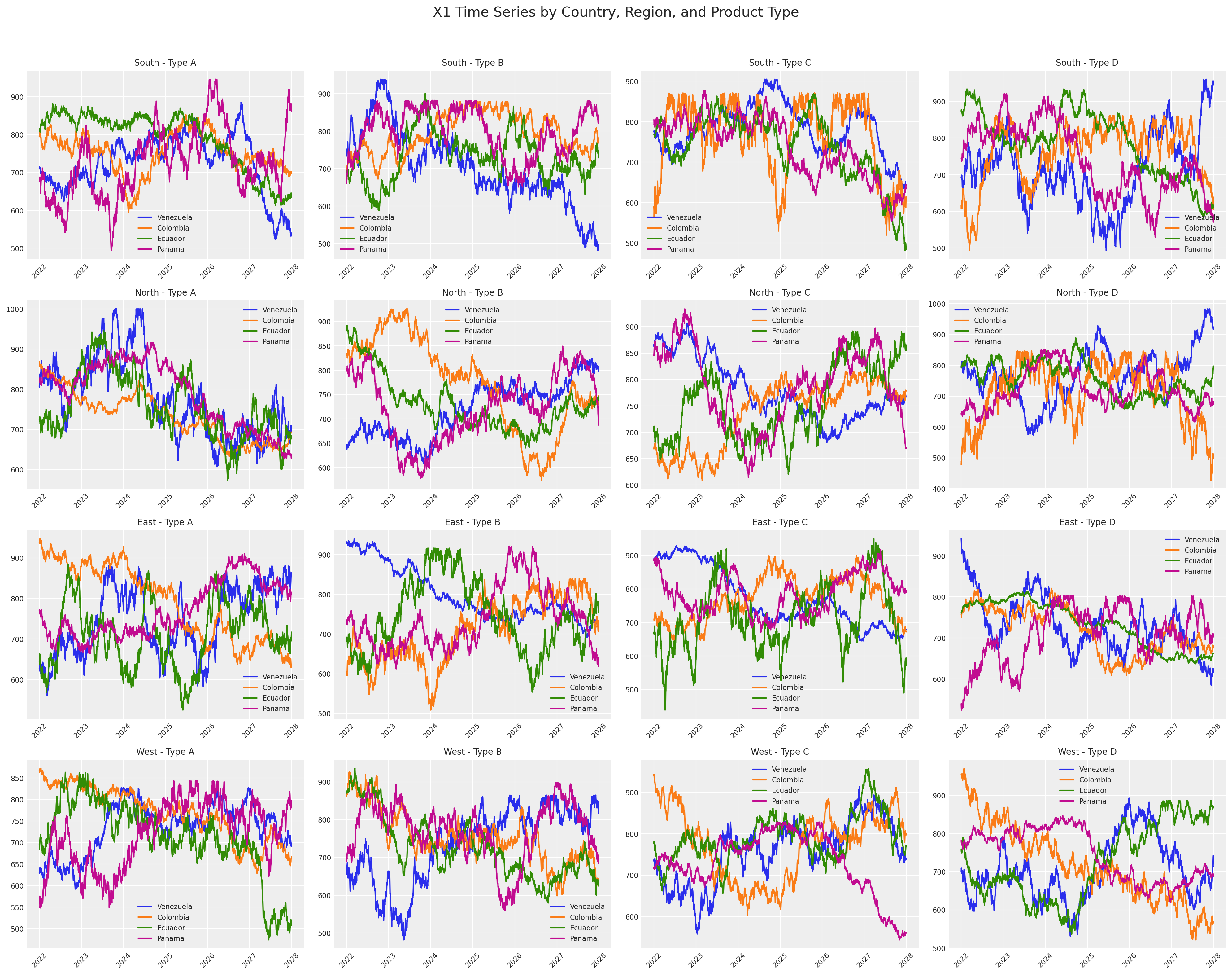
Now our dataset looks better, we have a time series with lenght day per each country, region and product type. Take a look to the number of time series only made for \(x1\).

# Create subplots for each combination of country, region, and product type
fig, axes = plt.subplots(4, 4, figsize=(20, 16))
fig.suptitle("X1 Time Series by Country, Region, and Product Type", fontsize=16, y=0.98)

for _, country in enumerate(countries):
    for j, (region, product_type) in enumerate(
        [(r, p) for r in regions for p in product_types]
    ):
        if j >= 16:  # Only plot first 16 combinations to fit in 4x4 grid
            break

        row = j // 4
        col = j % 4

        # Filter data for this specific combination using query syntax
        subset = multi_country_df.query(
            f"country == '{country}' and region == '{region}' and product_type == '{product_type}'"
        )

        if len(subset) > 0:  # Only plot if data exists
            subset = subset.set_index("date_week")
            axes[row, col].plot(subset.index, subset["x1"], label=f"{country}")
            axes[row, col].set_title(f"{region} - {product_type}", fontsize=10)
            axes[row, col].tick_params(axis="x", rotation=45, labelsize=8)
            axes[row, col].tick_params(axis="y", labelsize=8)
            axes[row, col].legend(fontsize=8)

plt.tight_layout(rect=[0, 0, 1, 0.96])
plt.show()

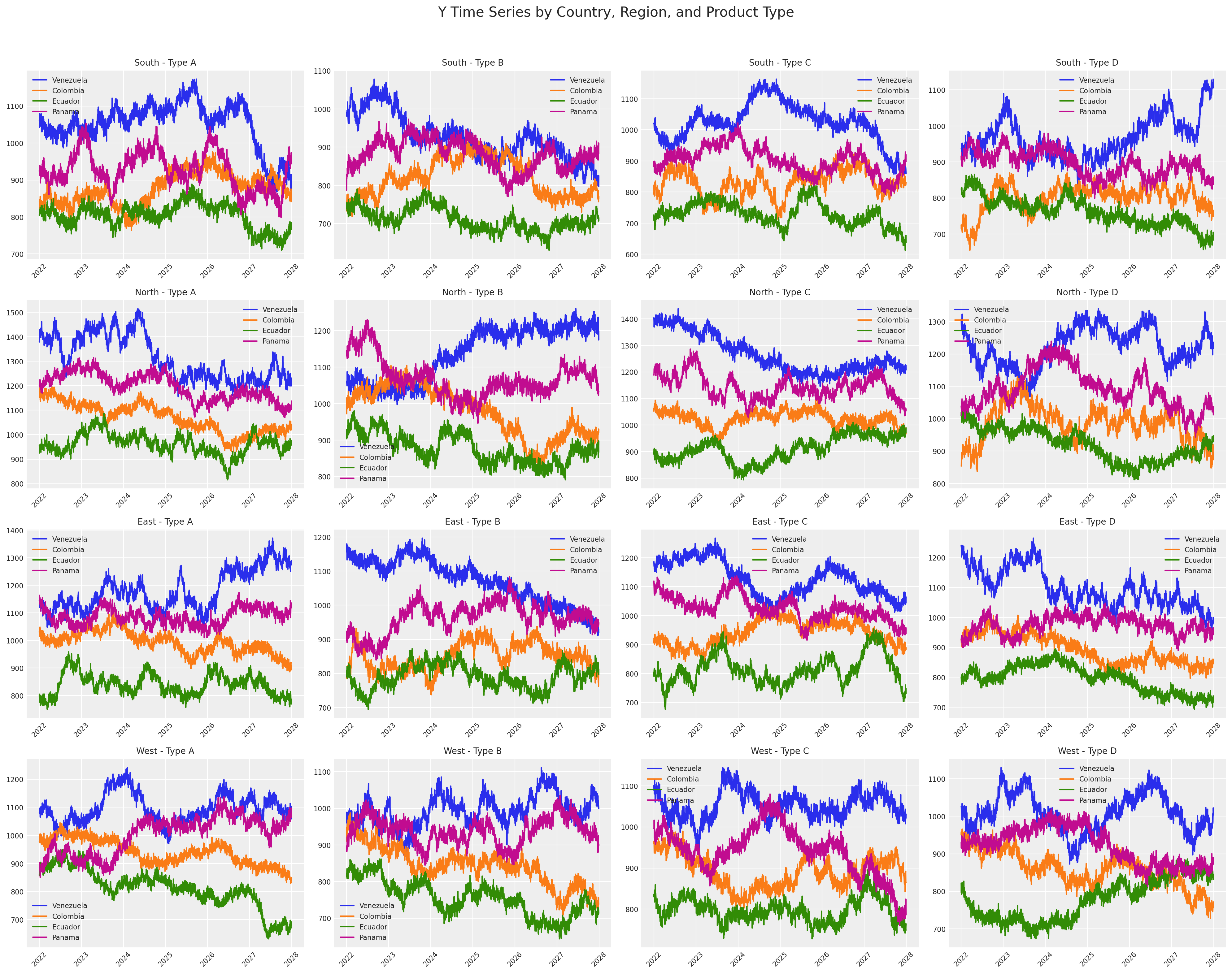
../../_images/5a1c37b8a49cd166b08fe979169a0bd717d95ec00591bb6a4c8faea2000f05fa.png

For each time series, we’ll make a linear combination as before to get a target variable!

# Define different coefficients, intercepts, and noise levels for each combination
combination_params = {}

# Create parameters for each combination of country, region, and product type
for country in countries:
    for region in regions:
        for product_type in product_types:
            # Create unique parameters for each combination
            base_coeffs = [0.5, 0.3, 0.2, 0.1]
            base_intercept = 100
            base_noise = 10

            # Add variation based on country
            country_multiplier = {
                "Venezuela": 1.2,
                "Colombia": 1.0,
                "Ecuador": 0.9,
                "Panama": 1.1,
            }[country]

            # Add variation based on region
            region_multiplier = {"North": 1.1, "South": 0.9, "East": 1.0, "West": 0.95}[
                region
            ]

            # Add variation based on product type
            product_multiplier = {
                "Type A": 1.05,
                "Type B": 0.95,
                "Type C": 1.0,
                "Type D": 0.98,
            }[product_type]

            # Calculate final parameters
            final_multiplier = (
                country_multiplier * region_multiplier * product_multiplier
            )

            combination_params[(country, region, product_type)] = {
                "coeffs": [c * final_multiplier for c in base_coeffs],
                "intercept": base_intercept * final_multiplier,
                "noise_std": base_noise
                * (final_multiplier * 0.5 + 0.5),  # Moderate noise variation
            }

# Initialize y column
multi_country_df["y"] = 0.0

# Calculate y for each combination with different parameters
for (country, region, product_type), params in combination_params.items():
    combination_mask = (
        (multi_country_df["country"] == country)
        & (multi_country_df["region"] == region)
        & (multi_country_df["product_type"] == product_type)
    )

    if combination_mask.sum() > 0:
        # Generate combination-specific noise
        combination_noise = np.random.normal(
            0, params["noise_std"], combination_mask.sum()
        )

        # Calculate y for this combination
        combination_y = (
            multi_country_df.loc[combination_mask, "x1"] * params["coeffs"][0]
            + multi_country_df.loc[combination_mask, "x2"] * params["coeffs"][1]
            + multi_country_df.loc[combination_mask, "x3"] * params["coeffs"][2]
            + multi_country_df.loc[combination_mask, "x4"] * params["coeffs"][3]
            + params["intercept"]
            + combination_noise
        )

        multi_country_df.loc[combination_mask, "y"] = combination_y

multi_country_df.head()

	date_week	country	region	product_type	x1	x2	x3	x4	y
0	2022-01-01	Venezuela	South	Type A	710.882064	957.721277	692.358987	647.460836	1060.700501
1	2022-01-02	Venezuela	South	Type A	713.843455	954.916067	683.856081	647.238756	1066.913341
2	2022-01-03	Venezuela	South	Type A	714.361066	952.231407	685.633316	646.582390	1041.857240
3	2022-01-04	Venezuela	South	Type A	713.603647	943.751500	690.015249	648.641505	1079.833391
4	2022-01-05	Venezuela	South	Type A	714.297808	939.881806	695.047680	650.883197	1067.399181

# Create subplots for each combination of country, region, and product type
fig, axes = plt.subplots(4, 4, figsize=(20, 16))
fig.suptitle("Y Time Series by Country, Region, and Product Type", fontsize=16)

for _, country in enumerate(countries):
    for j, (region, product_type) in enumerate(
        [(r, p) for r in regions for p in product_types]
    ):
        if j >= 16:  # Only plot first 16 combinations to fit in 4x4 grid
            break

        row = j // 4
        col = j % 4

        # Filter data for this specific combination
        # Filter data for this specific combination using query syntax
        subset = multi_country_df.query(
            f"country == '{country}' and region == '{region}' and product_type == '{product_type}'"
        )

        if len(subset) > 0:  # Only plot if data exists
            subset = subset.set_index("date_week")
            axes[row, col].plot(subset.index, subset["y"], label=f"{country}")
            axes[row, col].set_title(f"{region} - {product_type}", fontsize=10)
            axes[row, col].tick_params(axis="x", rotation=45, labelsize=8)
            axes[row, col].tick_params(axis="y", labelsize=8)
            axes[row, col].legend(fontsize=8)

plt.tight_layout(rect=[0, 0, 1, 0.96])
plt.show()

../../_images/7dbe4893c890efe0c0f0a66a001b53f64083dfe724ccc23d0a23fd7ec832bb40.png

Variational inference for High Dimensional grids#

We’ve already seen how dimensional design and MaskedPrior can shrink parameter space by excluding irrelevant combinations. However, there are regimes where this isn’t enough: as you add nonlinear transformations, trend/seasonality, multi-index structures, and custom effects, you can end up in very high-dimensional posterior geometries. In these cases, exact MCMC (e.g., NUTS) can become prohibitively expensive. This is where approximate inference shines. As Michael Betancourt aptly notes, “In high dimensions, expectations are the only thing that makes sense.” Approximations let you target informative summaries (e.g., posterior means, credible intervals) without paying the full cost of exact sampling.

PyMC-Marketing exposes PyMC’s variational and approximate methods directly, so you can switch from exact sampling to approximation with minimal code. For example, using ADVI via pm.fit(...) and then drawing samples from the approximation. This tool allows you to prototype and triage large models quickly. You can later escalate to full MCMC if the approximation looks adequate and the compute budget allows. For details on available approximation methods (e.g., ADVI, Full-Rank ADVI, SVGD), see the PyMC inference docs (search for “PyMC variational inference” and pm.fit).

Bias–variance trade-off: Variational families can underestimate posterior variance and miss correlations.
Pathologies in geometry: Multimodality, heavy tails, and strong curvature can break simple variational assumptions or lead to poor local optima.
Diagnostics matter: Monitor ELBO trajectories, check stability of solutions, and compare against short pilot NUTS runs on reduced models when possible.
Calibration risk: Downstream decisions (e.g., budget allocation) may be overconfident if variance is underestimated. Consider conservative policies or robust utilities.

_start_time = time.time()
linear_model.approximate_fit(
    X=df.drop(columns=["y"]),
    y=df["y"],
    fit_kwargs={"method": "advi"},  # goes to pm.fit(...)
    sample_kwargs={"draws": 1_000},  # goes to approximation.sample(...)
)
_end_time = time.time()
elapsed_time = _end_time - _start_time
print(f"Approximation took {elapsed_time:.2f} seconds")

Finished [100%]: Average Loss = 1,522.5

Approximation took 2.59 seconds

Final Thoughts#

What we’ve explored here is just a glimpse of what PyMC-Marketing can do. Beyond being a Marketing Mix Modeling toolkit, it’s a probabilistic modeling framework driven by PyMC that gives you the building blocks to design, extend, and experiment with Bayesian models of any complexity — from linear regressions to rich, hierarchical, time-aware systems.

PyMC-Marketing is not limited for marketing and more important you are not limited by templates. You can build, modify, and extend your models freely while standing on the solid foundation of PyMC’s probabilistic engine. Every additional layer — trend, seasonality, saturation, or custom effect — adds expressiveness without losing clarity or structure.

So, keep exploring! Try new transformations, mix causal and functional effects, benchmark inference strategies, and share your ideas with the community. If there’s a feature you wish existed — ask for it, or even better, help us build it.

PyMC-Marketing is evolving fast, and your curiosity is what drives its next step! 🔥

%reload_ext watermark
%watermark -n -u -v -iv -w

Last updated: Wed Oct 08 2025

Python implementation: CPython
Python version       : 3.12.11
IPython version      : 9.4.0

pandas        : 2.3.1
pytensor      : 2.31.7
matplotlib    : 3.10.3
pymc_marketing: 0.16.0
arviz         : 0.22.0
pymc_extras   : 0.4.0
pymc          : 5.25.1
xarray        : 2025.7.1
numpy         : 2.2.6

Watermark: 2.5.0

From Marketing Mix Models to Custom Bayesian GAMs: Extending PyMC-Marketing’s Core#

Introduction#

Import libraries#

Setting notebook#

Data generation process#

Sampler settings#

Simple Linear Model#

Adding additional dimensions into our additive model#

Creating hierarchical multidimensional model#

Adding Trend and Seasonality Components#

Custom functions in PyMC-Marketing#

Adding linear covariates#

Arbitrary terms in PyMC-Marketing#

Where are the GAMs?#

Recap: From Simple Lines to Complex Structures#

Parameter Growth & Sampling Time#

Excluding Variables from Sampling with `MaskedPrior`#

Variational inference for High Dimensional grids#

Final Thoughts#

From Marketing Mix Models to Custom Bayesian GAMs: Extending PyMC-Marketing’s Core#

Introduction#

Import libraries#

Setting notebook#

Data generation process#

Sampler settings#

Simple Linear Model#

Adding additional dimensions into our additive model#

Creating hierarchical multidimensional model#

Adding Trend and Seasonality Components#

Custom functions in PyMC-Marketing#

Adding linear covariates#

Arbitrary terms in PyMC-Marketing#

Where are the GAMs?#

Recap: From Simple Lines to Complex Structures#

Parameter Growth & Sampling Time#

Excluding Variables from Sampling with MaskedPrior#

Variational inference for High Dimensional grids#

Final Thoughts#

Excluding Variables from Sampling with `MaskedPrior`#